
Pump Affinity Laws: A Useful Shortcut That the System Can Overrule
Reduce a centrifugal pump from 100% speed to 80% speed and the familiar prediction is attractive: flow falls to 80%, head to 64% and shaft power to about 51%.
The equations are correct for corresponding points on geometrically similar pump curves under their stated assumptions. The common mistake is turning them into a promise about the installed system.
A variable-frequency drive changes the pump curve. It does not remove static head, change the pipework or force the operating point to remain at the same relative position on the curve. To predict actual flow and energy, the reduced-speed pump curve must meet the real system curve.
The three speed relationships
For the same rotodynamic pump and impeller diameter, the Hydraulic Institute presents the affinity relationships as:
Q₂ ÷ Q₁ = n₂ ÷ n₁
H₂ ÷ H₁ = (n₂ ÷ n₁)²
P₂ ÷ P₁ = (n₂ ÷ n₁)³
Where:
- Q is pump flow
- H is pump head
- P is pump input or shaft power
- n is rotational speed
These relationships assume that efficiency remains approximately constant between corresponding points. Real efficiency, motor loss and VFD loss can differ, particularly at low load.
A normalised example
Take a pump operating at:
- 100 m³/h
- 50 m head
- 20 kW shaft power
- 100% speed
The affinity-law estimates are:
| Speed | Corresponding flow | Corresponding head | Corresponding shaft power |
|---|---|---|---|
| 100% | 100 m³/h | 50.0 m | 20.00 kW |
| 90% | 90 m³/h | 40.5 m | 14.58 kW |
| 80% | 80 m³/h | 32.0 m | 10.24 kW |
| 70% | 70 m³/h | 24.5 m | 6.86 kW |
The power result explains the appeal of speed control. A 20% speed reduction produces an idealised shaft-power reduction of nearly 49%.
It does not follow that electrical input also falls by exactly 49%. Motor and VFD efficiency must be applied, and both vary with load and speed.
Why static head breaks the simple flow prediction
Imagine that the 100 m³/h duty requires:
- 25 m static head
- 25 m friction head
- 50 m total head
At 80% of design flow, the friction component would be approximately:
25 × 0.8² = 16 m
The system would therefore require:
25 + 16 = 41 m
But the affinity-law corresponding point at 80% speed produces only 32 m.
The pump cannot deliver the predicted 80 m³/h because 32 m is below the system requirement at that flow. The real operating point will be found where the full 80%-speed pump curve intersects the system curve, and it may be much farther left—or the pump may fail to meet the static lift at all.
In a closed circulating system with little or no static head, the system curve passes close to the origin. Under that condition, speed and flow often track more closely and the cube-law saving becomes a better first estimate.
A VFD controls speed, not duty
A pressure sensor, differential-pressure sensor, flow meter or process controller tells the VFD what speed to request. The control target decides where the system operates.
Holding a constant remote pressure may save more energy than holding a constant pressure at the pump discharge because the remote setpoint allows the drive to reduce head as flow falls. However, sensor placement and minimum equipment-pressure requirements must be verified.
For an HVAC loop, read why variable-speed control strategy matters more than motor speed alongside the affinity calculation. The curve and the control logic are two parts of the same decision.
Speed change and impeller trimming are not identical decisions
Affinity relationships are also used for limited changes in impeller diameter, but the approximation has constraints. Trimming changes the impeller geometry relative to the casing, clearances and vane shape. Efficiency does not necessarily remain constant.
The Hydraulic Institute advises staying within manufacturer recommendations and published curve limits. A trim may be a practical permanent correction for an oversized pump, but it is not a substitute for a new verified curve.
A VFD offers an adjustable curve and can follow variable demand. An impeller trim has no electronic drive loss and may be attractive where the required correction is permanent. The decision depends on the load profile, static head, control objective and required operating range.
Five checks before using the cube law in a saving estimate
1. Separate static and friction head
Write the system curve as a fixed component plus a flow-dependent component. If static head dominates, large speed reductions may not be possible.
2. Plot the reduced-speed pump curves
Do not scale only the design point. Scale several points from the manufacturer curve and find each intersection with the system curve.
3. Check efficiency rather than holding it constant
Read pump efficiency at the new operating point. Then apply motor and drive efficiency to estimate electrical input.
4. Check the manufacturer’s speed range
Minimum speed may be limited by motor cooling, bearing lubrication, seal behaviour, process requirements or the pump’s allowable operating region. Maximum speed can overload the motor and increase NPSHR.
5. Include every operating mode
One pump at full speed, two pumps at reduced speed and a standby-changeover condition can have different efficiencies. Sequence parallel pumps using composite curves rather than assuming each unit shares flow equally under every condition.
When the shortcut is genuinely useful
Affinity laws are excellent for:
- Building preliminary reduced-speed curves
- Testing whether a proposed VFD range is plausible
- Estimating the direction and scale of a power change
- Comparing speed control with throttling
- Identifying when static head will limit turndown
They are not a final guarantee of flow, pressure, efficiency or energy consumption.
For inline and multistage water duties, SHXINHUO’s ISG inline pumps and CDL vertical multistage pumps may be used with different control arrangements. Always use the current product curve and motor data when plotting speed limits.
The fastest way to misuse the affinity laws is to ask, “What happens to the pump at 80% speed?” The engineering question is, “Where does the 80%-speed pump curve meet this system curve, and what are the pump, motor and drive efficiencies there?”
Technical references
- Hydraulic Institute Data Tool — Pump Curves and Affinity Rules
- U.S. Department of Energy — Adjustable Speed Pumping Applications
- U.S. Department of Energy — Variable Speed Pumping: A Guide to Successful Applications
- Hydraulic Institute — Trimming Impellers to Reduce Energy Consumption
Data note
The normalised duty and static-head example are illustrative. The power values assume unchanged pump efficiency at corresponding points. Actual system flow and electrical power require the manufacturer curves, the system curve and motor/VFD performance data.