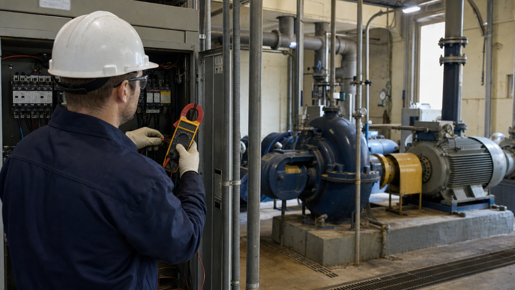
Pump Life-Cycle Cost: Turn Flow and Head into a Number the Buyer Can Use

Pump quotations make the purchase price easy to compare. Energy cost is harder to see because it arrives later, spread across thousands of operating hours.

That difference in visibility can distort a buying decision. A lower-priced pump that creates unnecessary head or operates at poor efficiency may cost more before its first planned overhaul. For a frequently used pump, the right comparison is not unit price against unit price. It is the cost of delivering the required service over the intended life.

The U.S. Department of Energy and Hydraulic Institute life-cycle-cost guidance treats energy, installation, operation, maintenance, downtime and disposal as parts of the same decision. Not every project needs a complex financial model, but every project can start with a transparent energy calculation.

The five inputs behind annual electricity cost

For a water pump, approximate electrical input power can be calculated as:

P input = ρ × g × Q × H ÷ η total

where:

• ρ is liquid density in kg/m³
• g is 9.81 m/s²
• Q is flow in m³/s
• H is total head in metres
• η total is the combined efficiency of pump, motor and drive

Annual electricity cost is:

Annual cost = P input × operating hours × electricity tariff

The calculation is only as good as its inputs. Use the normal operating point and annual load profile, not just the maximum design duty. Confirm whether efficiency is pump-only or includes the motor and drive.

Worked example: the cost of 10 m of wasted head

Consider a clean-water system that genuinely requires:

• Flow: 60 m³/h
• Total head: 40 m
• Operation: 4,000 hours per year
• Electricity tariff: $0.12/kWh

Two options are compared.

Option A: oversized pump with a throttling valve

• Pump develops 50 m at the required flow
• Excess 10 m is removed across the valve
• Combined efficiency at that operating point: 65%

Electrical input is approximately:

12.6 kW

Annual energy cost is:

12.6 × 4,000 × $0.12 = $6,048

Option B: pump matched to the system

• Pump develops the required 40 m
• Combined efficiency at the operating point: 78%

Electrical input is approximately:

8.4 kW

Annual energy cost is:

8.4 × 4,000 × $0.12 = $4,032

The difference is about $2,016 per year. Over ten years, the simple undiscounted difference is $20,160.

This is not a promise of savings for another project. It shows why 10 m of unnecessary head and a lower operating efficiency should be priced, not treated as harmless margin.

Why throttling is a cost, not a correction

A throttling valve increases system resistance and moves the operating point back along the pump curve. It can be a valid control method, especially in constant-flow or modest adjustment duties. The mistake is using permanent throttling to remove head that should never have been generated.

The pressure drop across the valve represents energy supplied by the pump and dissipated in the system. If the valve is routinely far closed, investigate:

• Whether the design head was overstated
• Whether several safety margins were added
• Whether the impeller can be trimmed
• Whether speed control suits the system curve
• Whether the pump should be replaced at the next planned outage

Do not reduce speed or trim an impeller without checking minimum head, operating region, power, NPSH and all required duties.

Model the load profile

The worked example uses one duty for 4,000 hours. Many systems need a better model.

A building booster set may operate at low demand overnight, moderate demand for most of the day and peak demand for short periods. An HVAC distribution pump may spend most of the season below design flow. A transfer pump may run at a relatively stable duty.

Divide the year into a small number of realistic operating bands:

Load band	Flow and head	Annual hours	Input kW	Annual kWh
Low	Measured or calculated	Hours	From curve/calculation	kW × hours
Normal	Measured or calculated	Hours	From curve/calculation	kW × hours
Peak	Measured or calculated	Hours	From curve/calculation	kW × hours

Add the annual kWh for each band, then apply the relevant tariff. This is usually more credible than multiplying peak motor power by total annual hours.

Include demand charges and local tariff structure

Some electricity bills charge for both energy use in kWh and peak electrical demand in kW. Time-of-use rates may also apply. A pump that starts during a facility peak can affect cost differently from one that runs off-peak.

For a preliminary international comparison, a single energy tariff is understandable. For an investment decision, use the customer’s bill structure and local currency. State whether taxes, demand charges and escalation are included.

Life-cycle cost is broader than electricity

The life-cycle-cost equation is commonly expressed as the sum of:

• Initial purchase cost
• Installation and commissioning
• Energy
• Operation
• Maintenance and repair
• Downtime or lost production
• Environmental cost
• Decommissioning and disposal

These terms do not all need the same level of precision. The purpose is to expose important differences.

A more efficient pump may need a higher initial budget. A pump with easier seal or bearing access may reduce maintenance labour. A duty/standby arrangement may cost more upfront but avoid unacceptable downtime. A product that requires a special spare from another continent may carry a practical inventory cost.

Write the assumptions beside the result. A single total without its assumptions looks precise but is difficult to audit.

What changes the result fastest?

In most simple energy models, four items deserve a sensitivity check:

Operating hours. A small efficiency difference matters little for a pump used 50 hours a year and much more for one used 6,000 hours.

Electricity tariff. Use a realistic current tariff and test a higher value for a long project life.

Actual duty. An incorrectly estimated flow or head can outweigh a small difference in catalogue efficiency.

Part-load control. Variable speed can reduce power substantially in friction-dominated variable-flow systems, but systems with large static head need a full curve analysis.

Calculate a low, expected and high case. Decision-makers can then see which assumptions deserve measurement before purchase.

A practical quotation request

Ask competing suppliers to return the same data at the same duties:

1. Flow and total head
2. Pump efficiency
3. Shaft power
4. Motor and drive efficiency
5. Expected electrical input
6. NPSH3
7. Permitted operating region
8. Materials and seal arrangement
9. Maintenance interval assumptions
10. Recommended spare parts

SHXINHUO’s centrifugal pump range covers clean-water circulation, transfer and boosting duties. For a meaningful energy comparison, provide the expected operating hours and several load points along with the peak requirement.

The cheapest pump to buy and the cheapest pumping service are not always the same product. Once wasted head is translated into kWh and annual cost, that difference becomes much easier to discuss.

Technical references

• U.S. Department of Energy — Pump Life Cycle Costs: Executive Summary
• U.S. Department of Energy — Pump Systems Resources
• Hydraulic Institute — Calculate Pump System Energy Costs

Data note

The example assumes water, steady operation, a constant $0.12/kWh tariff and no demand charges, escalation or discounting. Values are rounded. Replace every assumption with project data before making an investment decision.